cs224n Lecture Notes 1

Keyphrases:

Natural Language Processing. Word Vectors. Singular Value Decomposition. Skip-gram. Continuous Bag of Words (CBOW). Negative Sampling. Hierarchical Softmax. Word2Vec.

description: This set of notes begins by introducing the concept of Natural Language Processing (NLP) and the problems NLP faces today. We then move forward to discuss the concept of representing words as numeric vectors. Lastly, we discuss popular approaches to designing word vectors.

---

Table of Contents

• Introduction to Natural Language Processing
• Iteration Based Methods - Word2vec
  • Language Models (Unigrams, Bigrams, etc.)
  • Continuous Bag of Words Model (CBOW)
  • Skip-Gram Model
  • Negative Sampling
  • Hierarchical Softmax

Introduction to Natural Language Processing

Examples of tasks

Easy

• Spell Checking
• Keyword Search
• Finding Synonyms

Medium

• Parsing information from websites, documents, etc.

Hard

• Machine Translation (e.g. Translate Chinese text to English)

• Semantic Analysis (What is the meaning of query statement?)

• Coreference (e.g. What does “he” or “it” refer to given a document?)

• Question Answering (e.g. Answering Jeopardy questions)

Iteration Based Methods - Word2vec

Instead of computing and storing global information about some huge dataset (which might be billions of sentences), we can try to create a model that will be able to learn one iteration at a time and eventually be able to encode the probability of a word given its context.

Language Models (Unigrams, Bigrams, etc.)

The probability on any given sequence of n words:

$$P(w_1, w_2,..., w_n)$$

Bigram model:

$$P(w_1, w_2,..., w_n) = \prod_{i=2}^{n}P(w_i|w_{i-1})$$

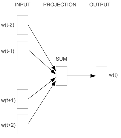
Continuous Bag of Words Model (CBOW)

Predicting a center word from the surrounding context.

Notation for CBOW Model:

• $w_i$: Word i from vocabulary V
• $V\in R^{n\times\mid V\mid}$: Input word matrix
• $v_i$: i-th column of V, the input vector representation of word $w_i$
• $U\in R^{\mid V\mid\times n}$: Output word matrix
• $u_i$: i-th row of U, the output vector representation of word $w_i$

1. We generate our one hot word vectors for the input context $(x^{c-m},…,x^{c-1},x^{c+1},…x^{c+m} \in R^{\mid V\mid})$
2. We get our embedded word vectors for the context $(v_{c-m}=Vx^{c-m},…,v_{c+m}=Vx^{c+m} \in R^{n})$
3. Average these vectors to get $\hat{v} = \frac{v_{c-m}+…+v_{c+m}}{2m}$
4. Generate a score vector $z=U\hat{v}\in R^{\mid V\mid}$
5. Turn the scores into probabilities $\hat{y}=softmax(z)\in R^{\mid V\mid}$

$$minimize J = -logP(w_c|w_{c-m},...,w_{c+m}) = -logP(u_c|\hat{v}) = -log\frac{exp(u_c^T\hat{v})}{\sum_{j=1}^{\mid V\mid}exp(u_j^T\hat{v})}$$

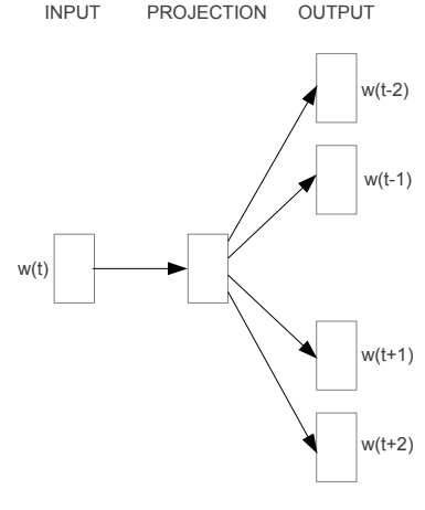
Skip-Gram Model

Predicting surrounding context words given a center word.

1. We generate our one hot input vector $(x \in R^{\mid V\mid})$ of the center word
2. We get our embedded word vectors for the context $(v_c=Vx \in R^{n})$
3. Generate a score vector $z=Uv_c$
4. Turn the scores into probabilities $\hat{y}=softmax(z)\in R^{\mid V\mid}$.note that $(\hat{y}{c-m},…,\hat{y}{c-1},\hat{y}{c+1},…\hat{y}{c+m})$ are the probabilities of observing each context word

Assumption:given the center word, all output words are completely independent

$$minimize J = -logP(w_{c-m},...,w_{c+m}|w_c) = -log\prod_{j=0,j\ne m}^{2m}P(u_{c-m+j}|v_c)$$

Negative Sampling

Note that the summation over $\mid V\mid$ is computationally huge.A simple idea is we could instead just approximate it.We “sample” from a noise distribution $P_n(w)$ whose probabilities match the ordering of the frequency of the vocabulary.

Let’s denote by $P(D = 1\mid w,c)$ the probability that (w, c) came from the corpus data and model $P(D = 1\mid w,c)$ with the sigmoid function:

$$P(D = 1\mid w,c,\theta) = \sigma(v_c^Tv_w)$$

We take a simple maximum likelihood approach of these two probabilities. (Here we take $\theta$ to be the parameters of the model, and in our case it is V and U.)

$$\theta = argmax_{\theta}\prod_{(w,c)\in D}P(D=1\mid w,c,\theta)\prod_{(w,c)\in \hat{D}}P(D=0\mid w,c,\theta) = argmax_{\theta}\sum_{(w,c)\in D}\sigma(u_w^Tv_c) + \sum_{(w,c)\in \hat{D}}\sigma(-u_w^Tv_c)$$

We can generate $\hat(D)$ on the fly by randomly sampling this negative from the word bank.

Hierarchical Softmax

In practice, hierarchical softmax tends to be better for infrequent words, while negative sampling works better for frequent words and lower dimensional vectors

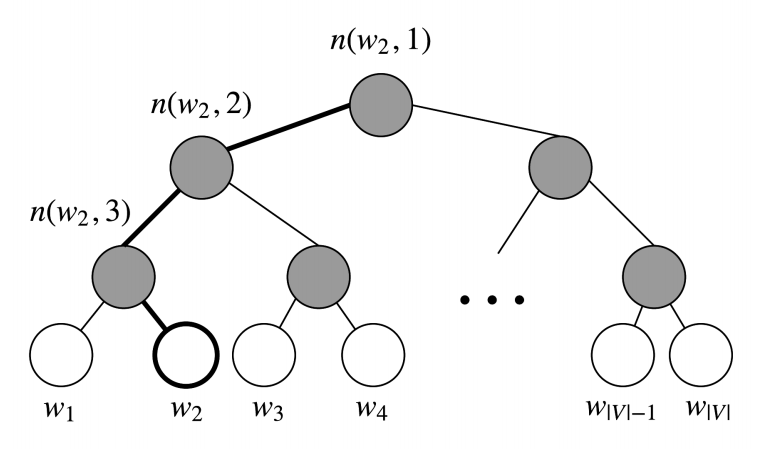
Hierarchical softmax uses a binary tree to represent all words in the vocabulary. Each leaf of the tree is a word, and there is a unique path from root to leaf. In this model, there is no output representation for words. Instead, each node of the graph (except the root and the leaves) is associated to a vector that the model is going to learn.

In this model, the probability of a word w given a vector $w_i$, $P(w\mid w_i)$, is equal to the probability of a random walk starting in the root and ending in the leaf node corresponding to w. The main advantage in computing the probability this way is that the cost is only $O(log(\mid V\mid))$, corresponding to the length of the path.

we can compute the probability as

$$P(w\mid w_i) = \prod_{j=1}^{L(w)-1}\sigma([n(w,j+1)=ch(n(w,j))]v_{n(w,j)}^Tv_{w_i})$$ $$[x] = \begin{cases} 1, & \text{if $x$ is true} \\ -1, & \text{otherwise} \end{cases}$$

$[x]$ term provides normalization because $\sigma(x)+\sigma(-x)=1$

The speed of this method is determined by the way in which the binary tree is constructed and words are assigned to leaf nodes.Mikolov et al. use a binary Huffman tree, which assigns frequent words shorter paths in the tree.