Complete Guide to Parameter Tuning in GBM

Table of Contents

1. How Boosting Works
2. Understanding GBM Parameters
3. Tuning Parameters

1. How Boosting Works

Boosting is a sequential technique which works on the principle of ensemble. It combines a set of weak learners and delivers improved prediction accuracy. At any instant t, the model outcomes are weighed based on the outcomes of previous instant t-1. The outcomes predicted correctly are given a lower weight and the ones miss-classified are weighted higher.

2. GBM Parameters

The overall parameters can be divided into 3 categories:

1. Tree-Specific Parameters: These affect each individual tree in the model.
2. Boosting Parameters: These affect the boosting operation in the model.
3. Miscellaneous Parameters: Other parameters for overall functioning.

2.1 Tree-Specific Parameters

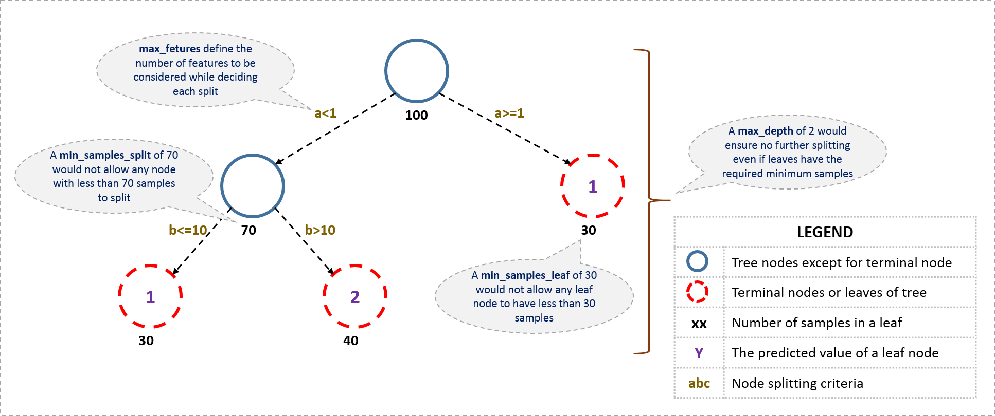
1. min_samples_split
   • Defines the minimum number of samples (or observations) which are required in a node to be considered for splitting.
   • Used to control over-fitting. Higher values prevent a model from learning relations which might be highly specific to the particular sample selected for a tree.
   • Too high values can lead to under-fitting hence, it should be tuned using CV.
2. min_samples_leaf
   • Defines the minimum samples (or observations) required in a terminal node or leaf.
   • Used to control over-fitting similar to min_samples_split.
   • Generally lower values should be chosen for imbalanced class problems because the regions in which the minority class will be in majority will be very small.
3. min_weight_fraction_leaf
   • Similar to min_samples_leaf but defined as a fraction of the total number of observations instead of an integer.
   • Only one of #2 and #3 should be defined.
4. max_depth
   • The maximum depth of a tree.
   • Used to control over-fitting as higher depth will allow model to learn relations very specific to a particular sample.
   • Should be tuned using CV.
5. max_leaf_nodes
   • The maximum number of terminal nodes or leaves in a tree.
   • Can be defined in place of max_depth. Since binary trees are created, a depth of ‘n’ would produce a maximum of 2^n leaves.
   • If this is defined, GBM will ignore max_depth.
6. max_features
   • The number of features to consider while searching for a best split. These will be randomly selected.
   • As a thumb-rule, square root of the total number of features works great but we should check upto 30-40% of the total number of features.
   • Higher values can lead to over-fitting but depends on case to case.

2.2 Boosting Parameters

1. learning_rate
   • This determines the impact of each tree on the final outcome. GBM works by starting with an initial estimate which is updated using the output of each tree. The learning parameter controls the magnitude of this change in the estimates.
   • Lower values are generally preferred as they make the model robust to the specific characteristics of tree and thus allowing it to generalize well.
   • Lower values would require higher number of trees to model all the relations and will be computationally expensive.
2. n_estimators
   • The number of sequential trees to be modeled.
   • Though GBM is fairly robust at higher number of trees but it can still overfit at a point. Hence, this should be tuned using CV for a particular learning rate.
3. subsample
   • The fraction of observations to be selected for each tree. Selection is done by random sampling.
   • Values slightly less than 1 make the model robust by reducing the variance.
   • Typical values ~0.8 generally work fine but can be fine-tuned further.

2.3 Miscellaneous Parameters

1. loss
   • It refers to the loss function to be minimized in each split.
   • It can have various values for classification and regression case. Generally the default values work fine. Other values should be chosen only if you understand their impact on the model.
2. init
   • This affects initialization of the output.
   • This can be used if we have made another model whose outcome is to be used as the initial estimates for GBM.
3. random_state
   • The random number seed so that same random numbers are generated every time.
   • This is important for parameter tuning. If we don’t fix the random number, then we’ll have different outcomes for subsequent runs on the same parameters and it becomes difficult to compare models.
   • It can potentially result in overfitting to a particular random sample selected. We can try running models for different random samples, which is computationally expensive and generally not used.
4. verbose
   • The type of output to be printed when the model fits. The different values can be:
   • 0: no output generated (default)
   • 1: output generated for trees in certain intervals
   • >1: output generated for all trees
5. warm_start
   • This parameter has an interesting application and can help a lot if used judicially.
   • Using this, we can fit additional trees on previous fits of a model. It can save a lot of time and you should explore this option for advanced applications
6. presort
   • Select whether to presort data for faster splits.
   • It makes the selection automatically by default but it can be changed if needed.

3. Tuning Parameters

3.1 General Approach for Parameter Tuning

As discussed earlier, there are two types of parameter to be tuned here – tree based and boosting parameters. There are no optimum values for learning rate as low values always work better, given that we train on sufficient number of trees.

Though, GBM is robust enough to not overfit with increasing trees, but a high number for pa particular learning rate can lead to overfitting. But as we reduce the learning rate and increase trees, the computation becomes expensive and would take a long time to run on standard personal computers.

Keeping all this in mind, we can take the following approach:

1. Choose a relatively high learning rate. Generally the default value of 0.1 works but somewhere between 0.05 to 0.2 should work for different problems
2. Determine the optimum number of trees for this learning rate. This should range around 40-70. Remember to choose a value on which your system can work fairly fast. This is because it will be used for testing various scenarios and determining the tree parameters.
3. Tune tree-specific parameters for decided learning rate and number of trees. Note that we can choose different parameters to define a tree and I’ll take up an example here.
4. Lower the learning rate and increase the estimators proportionally to get more robust models.

3.2 Fix learning rate and number of estimators for tuning tree-based parameters

we need to set some initial values of other parameters

1. min_samples_split = 500 : This should be ~0.5-1% of total values. Since this is imbalanced class problem, we’ll take a small value from the range.
2. min_samples_leaf = 50 : Can be selected based on intuition. This is just used for preventing overfitting and again a small value because of imbalanced classes.
3. max_depth = 8 : Should be chosen (5-8) based on the number of observations and predictors. This has 87K rows and 49 columns so lets take 8 here.
4. max_features = ‘sqrt’ : Its a general thumb-rule to start with square root.
5. subsample = 0.8 : This is a commonly used used start value.

we can do a grid search and test out values from 20 to 80 in steps of 10.

#Choose all predictors except target & IDcols
predictors = [x for x in train.columns if x not in [target, IDcol]]
param_test1 = {'n_estimators':range(20,81,10)}
gsearch1 = GridSearchCV(estimator = GradientBoostingClassifier(learning_rate=0.1, min_samples_split=500,min_samples_leaf=50,max_depth=8,max_features='sqrt',subsample=0.8,random_state=10), 
param_grid = param_test1, scoring='roc_auc',n_jobs=4,iid=False, cv=5)
gsearch1.fit(train[predictors],train[target])

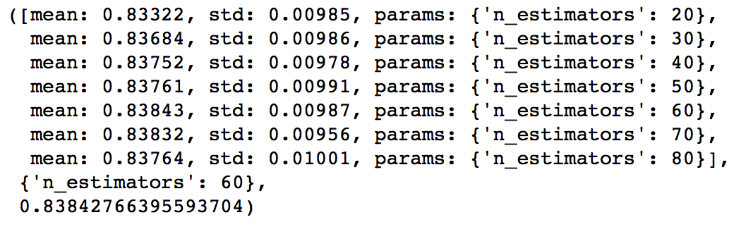
The output can be checked using following command:

gsearch1.grid_scores_, gsearch1.best_params_, gsearch1.best_score_

3.3 Tuning tree-specific parameters

Now lets move onto tuning the tree parameters

1. max_depth and num_samples_split
2. min_samples_leaf
3. max_features
4. subsample
5. n_estimators

The order of tuning variables should be decided carefully. You should take the variables with a higher impact on outcome first. For instance, max_depth and min_samples_split have a significant impact and we’re tuning those first.